I'm decoding motor imagery from EEG, classical pipeline first, deep models later. BCI Competition IV Dataset 2a is the de facto dataset for benchmarking motor decoding algorithms.
My results -> 0.621 ± 0.154 average across 9 subjects
The dataset
It includes:
- 9 different subjects
- A cue-based 4-class Motor Imagery task (left hand, right hand, both feet, tongue)
- 22 electrodes covering the motor cortex
- 576 4-second trials split evenly for training and testing (288 for training, 288 for testing)
- Sampled at 250Hz
Each subject has one training session and one test session, recorded on different days. The cue lands at ; the imagery period runs from roughly to after. The day-gap between sessions matters later — keep it in mind.
Preprocessing
EEG channels only, bandpass 8–30 Hz, epoch from to around each cue with a baseline.
eeg = run_raw.copy().pick("eeg").filter(l_freq=8.0, h_freq=30.0)
events, ev_id = mne.events_from_annotations(eeg)
epochs = mne.Epochs(eeg, events, event_id=class_ids,
                    tmin=-0.5, tmax=4.0, baseline=(-0.5, 0),
                    preload=True)
The 8–30 Hz band isn't a tunable hyperparameter — it's the mu (8–13 Hz) and beta (13–30 Hz) ranges where motor imagery actually lives.
- <8 Hz is mostly slow drift and ocular artifacts
- >30 Hz is mostly muscle noise.
One session out: a tensor of shape (n_trials, 22, 1126), where .
CSP, with the actual math
CSP (Common Spatial Patterns) finds spatial filters — linear combinations of the 22 channels — that maximize the variance of one class while minimizing the variance of the other. Since the 8–30 Hz bandpass is already applied, post-filter variance is band power, which is exactly the signal ERD lives in.
If you're interested, I wrote a more detailed outline here -> Common Spatial Patterns guide.
For two classes with covariance matrices and , CSP solves the generalized eigenvalue problem:
The eigenvalue is the share of total variance the filter assigns to class 1. The largest eigenvectors are the strongest "class 1 vs rest" directions; the smallest are the strongest "class 2 vs rest" directions. I take the top and bottom to get spatial filters per binary problem.
T = X.shape[2]
cov1 = (X[y == 0] @ X[y == 0].transpose(0, 2, 1)).mean(0) / (T - 1)
cov2 = (X[y == 1] @ X[y == 1].transpose(0, 2, 1)).mean(0) / (T - 1)
_, V = eigh(cov1, cov1 + cov2)
filters = np.concatenate([V[:, :k], V[:, -k:]], axis=1).T  # (2k, C)
Features: log of normalized variance
Filtering a trial gives of shape (2k, T). Each filter collapses to one number via variance over time, then I take the log of the normalized variance:
Normalization removes per-trial scale; the log pushes the distribution toward Gaussian, which is exactly what an LDA wants downstream.
Z = filters @ X                # (N, 2k, T)
v = (Z ** 2).mean(axis=2)      # (N, 2k)
features = np.log(v / v.sum(axis=1, keepdims=True))
Multi-class via one-vs-rest
CSP is binary by definition. For the four-class 2a problem I fit one CSP per class against the rest and concatenate the feature blocks:
features = np.concatenate(
    [csp_c.transform(X) for csp_c in csps_per_class],
    axis=1
)  # shape (N, num_classes * 2k)
Joint-diagonalization variants exist and probably do better on 2a, but one-vs-rest is the right baseline.
LDA, also a generalized eigenvalue problem
CSP gives me a feature vector per trial. I need a classifier. Fisher's linear discriminant — closed-form, no hyperparameters, and structurally the same problem as CSP itself.
Fisher's objective: find a direction such that the projected class means are as separated as possible relative to the within-class scatter. With
the optimal projection solves
A generalized Rayleigh quotient. CSP was one of these. So is LDA. The two halves of my pipeline are the same structural problem solved with different scatter matrices — and both reduce to generalized eigenvalue problems of the form .
For two classes, the closed form collapses to:
For four classes I use the Gaussian-with-shared-covariance form. Each class gets a discriminant function
and the predicted class is . Those terms come from the log of the Gaussian density : expanding the Mahalanobis quadratic gives
The piece together with the normalization drop out because they don't depend on . The remaining is the log of the class prior — the marginal probability before seeing , estimated here from class frequencies in the training set. (This dataset is class-balanced, so for all .)
The shared-covariance assumption is doing real work — it's why the quadratic-in- terms cancel and the decision boundaries are linear. For CSP features it's defensible: they're log-normalized variances of band-limited signals, so per-class covariances tend to be comparable in scale.
def predict(self, X):
    scores = (X @ self.cov_inv_ @ self.means_.T
              - 0.5 * (self.means_ @ self.cov_inv_ * self.means_).sum(axis=1)
              + np.log(self.priors_))
    return self.classes_[np.argmax(scores, axis=1)]
I wrote LDA from scratch rather than calling sklearn. The predictions match LinearDiscriminantAnalysis(solver="lsqr") to floating-point precision on this dataset.
Evaluating it — and the leak I almost shipped
First protocol: grid search over CSP component count and a couple of other knobs, evaluate each configuration on the held-out test set, pick the best per subject. The numbers looked good.
Then I noticed what I was actually doing. No individual model was trained on the test set, true — but the selection step was reading test accuracy and choosing which model to call mine. Test data had informed the pipeline. Any number I reported would be biased upward by an unknown amount.
The fix is the standard protocol, but worth being explicit about:
- For each subject, 5-fold
StratifiedKFoldon the training session, withshuffle=True, random_state=42, to evaluate every hyperparameter configuration. CSP and LDA refit inside each fold. - Pick the configuration with the best CV mean. Refit the full pipeline on all of the training session with those hyperparameters.
- Evaluate once on the test session. One number. No re-tuning.
The refit-inside-each-fold detail is the easy one to miss. If I fit CSP once on all the training data and reused it across folds, the spatial filters would have seen the validation trials before they were ever predicted on. Subtler than the headline leak; same category of error.
skf = StratifiedKFold(n_splits=5, shuffle=True, random_state=42)
for hp in grid:
    fold_scores = []
    for tr, va in skf.split(X_train, y_train):
        csp = CSP(**hp).fit(X_train[tr], y_train[tr])
        lda = LDA().fit(csp.transform(X_train[tr]), y_train[tr])
        fold_scores.append((lda.predict(csp.transform(X_train[va])) == y_train[va]).mean())
    cv_results[hp] = (np.mean(fold_scores), np.std(fold_scores))
The biggest thing I built at Level 1 wasn't either model — it was an evaluation harness I can trust the numbers from.
Results
Per-subject test accuracy after the fix:
| Subject | Best | CV mean ± std | Test | CV → Test gap |
|---|---|---|---|---|
| A01 | 2 | 0.789 ± 0.064 | 0.691 | +0.098 |
| A02 | 4 | 0.583 ± 0.028 | 0.476 | +0.107 |
| A03 | 3 | 0.882 ± 0.045 | 0.785 | +0.097 |
| A04 | 5 | 0.614 ± 0.033 | 0.517 | +0.097 |
| A05 | 2 | 0.469 ± 0.038 | 0.403 | +0.066 |
| A06 | 4 | 0.500 ± 0.066 | 0.434 | +0.066 |
| A07 | 3 | 0.775 ± 0.083 | 0.781 | −0.006 |
| A08 | 2 | 0.861 ± 0.048 | 0.819 | +0.042 |
| A09 | 5 | 0.840 ± 0.026 | 0.681 | +0.159 |
Cross-subject mean: 0.621 ± 0.154.
Published CSP+LDA baselines on 2a generally fall in the 0.55–0.70 band depending on preprocessing and multiclass scheme. My number sits in the middle of that. I haven't beaten anything; I've reproduced the baseline.
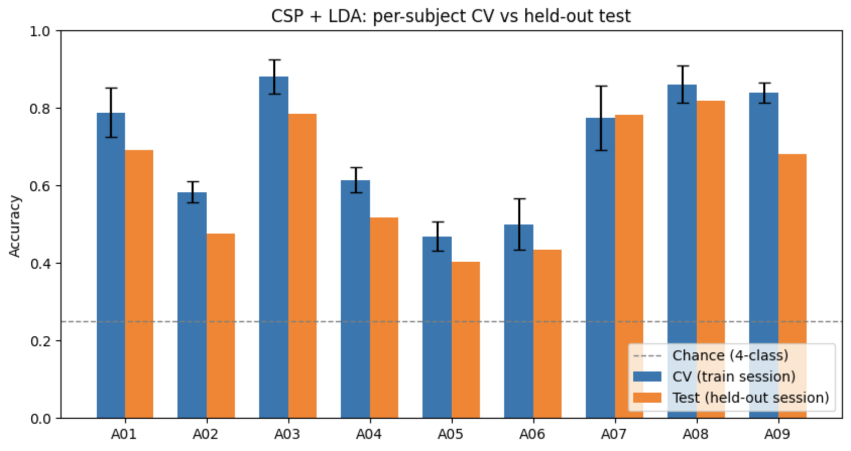
Two things worth pulling out.
The CV-to-test gap. Across subjects, CV mean overshoots test accuracy by roughly 8 percentage points on average. Training and test sessions were recorded on different days. Different impedances, different cap placement, different attentional state. 5-fold CV samples both train and validation from inside one session, so it never crosses that distribution boundary; the held-out test does. The gap is the cost of session-to-session shift, made visible.
Subject variance. Some subjects clear 0.80; the bottom pair (A05, A06) sit in the low 0.40s — well above chance (0.25) but too low to be useful. BCI illiteracy is a real phenomenon — roughly 15–30% of subjects produce MI signals that classical pipelines cannot separate, regardless of model tuning. It's not a bug at Level 1; it's a fact about the population.
Pooled across all 9 subjects (2,592 test trials), rows are the true class and columns the prediction:
| True ↓ / Pred → | Left hand | Right hand | Both feet | Tongue |
|---|---|---|---|---|
| Left hand | 422 | 124 | 59 | 43 |
| Right hand | 115 | 428 | 57 | 48 |
| Both feet | 61 | 69 | 397 | 121 |
| Tongue | 48 | 121 | 117 | 362 |
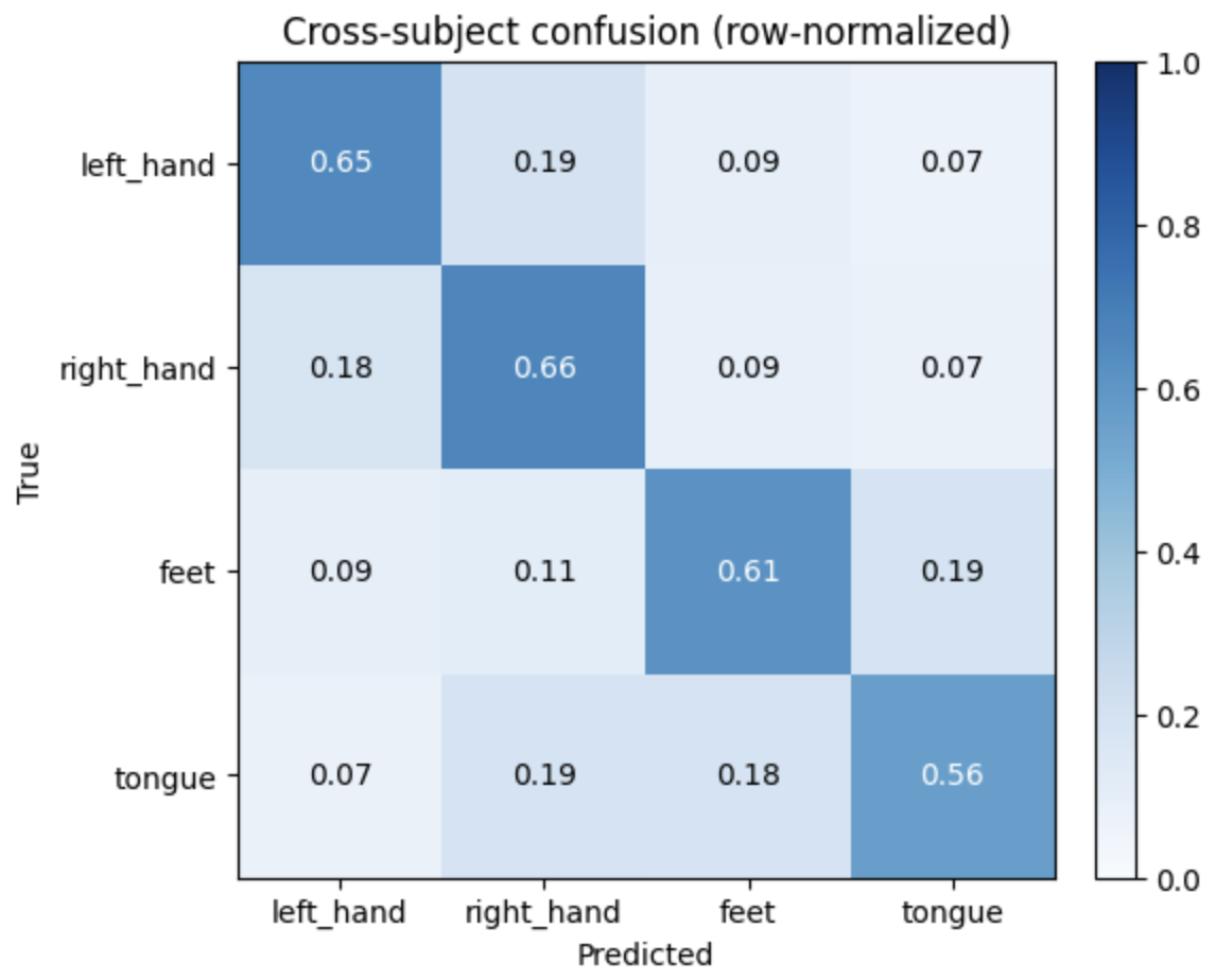
The clearest pattern is left↔right hand confusion (124 and 115 off-diagonal) — same rhythms, mirrored cortex, and CSP can blur the lateralization for some subjects. Beyond that the errors are diffuse: feet and tongue confuse with each other (~120 each direction) but also leak heavily into the hand classes. The motor-homunculus story is real for hands; it's a much weaker organizing principle for the rest.
What I'm taking into Level 2
A few honest gaps I'm carrying forward.
My CSP is a simplified variant. No per-trial demeaning, no trace normalization. The canonical Blankertz et al. 2008 formulation does both. At single-band 8–30 Hz with trials, the difference is small enough that I land in the published range. At Level 2 (FBCSP) it stops being optional — multiple bands with varying amplitudes mean trace normalization is doing real stabilization work.
The 8–30 Hz band is wide. Mu (8–13) and beta (13–30) are physiologically distinct rhythms with different spatial signatures. A single CSP per binary problem averages across that. FBCSP — Level 2 — fixes this by learning per-sub-band filters and selecting the discriminative ones.
Session shift is the open problem. That ~8pt CV-to-test gap is the structural ceiling on any model that trains within one session and evaluates on another. It's not obvious that adding parameters helps — deep models can also overfit to session-specific statistics. Level 3 (EEGNet) will give me an empirical answer rather than a theoretical one.